
Engineers Approach to Aging
Energy Landscape of Life

It would come as no surprise that organisms are not static blueprints. An organism is a closed-loop control system that maintains homeostasis via feedback and communication with its constituent parts. Whether its breakage of the DNA, external stress from UV light, or metabolism, living systems are constantly being pushed away from stable equilibrium. Each molecule or a cell only knows its local rules, but the whole organism behaves in a coherent way, converging towards preferred configuration. Our organism consists of trillions of these parts, and how can we hope to disentangle something as complex as aging?
Aging is usually studied as a collection of molecular events that lead to organismal failure. Here, I will take a different view by looking at life as a dynamical system with attractors where homeostasis represents trajectories flowing into a stable basin in state space.
My core hypothesis is that aging is a gradual flattening of the organism’s developmental attractor which constitutes loss of curvature, loss of restoring forces, and drift away from youthful setpoint.
We can visualize this with the classic “ball-in-a-basin” metaphor. Formally we could map all possible cellular configurations (epigenetic, transcriptomic, physiological, etc.) and assign each an energy value proportional to how unlikely or unstable it is. Youth corresponds to a landscape with high curvature and low entropy (a narrow valley with a clear direction towards homeostasis), while aged systems sit in flatter, lower-curvature surfaces.
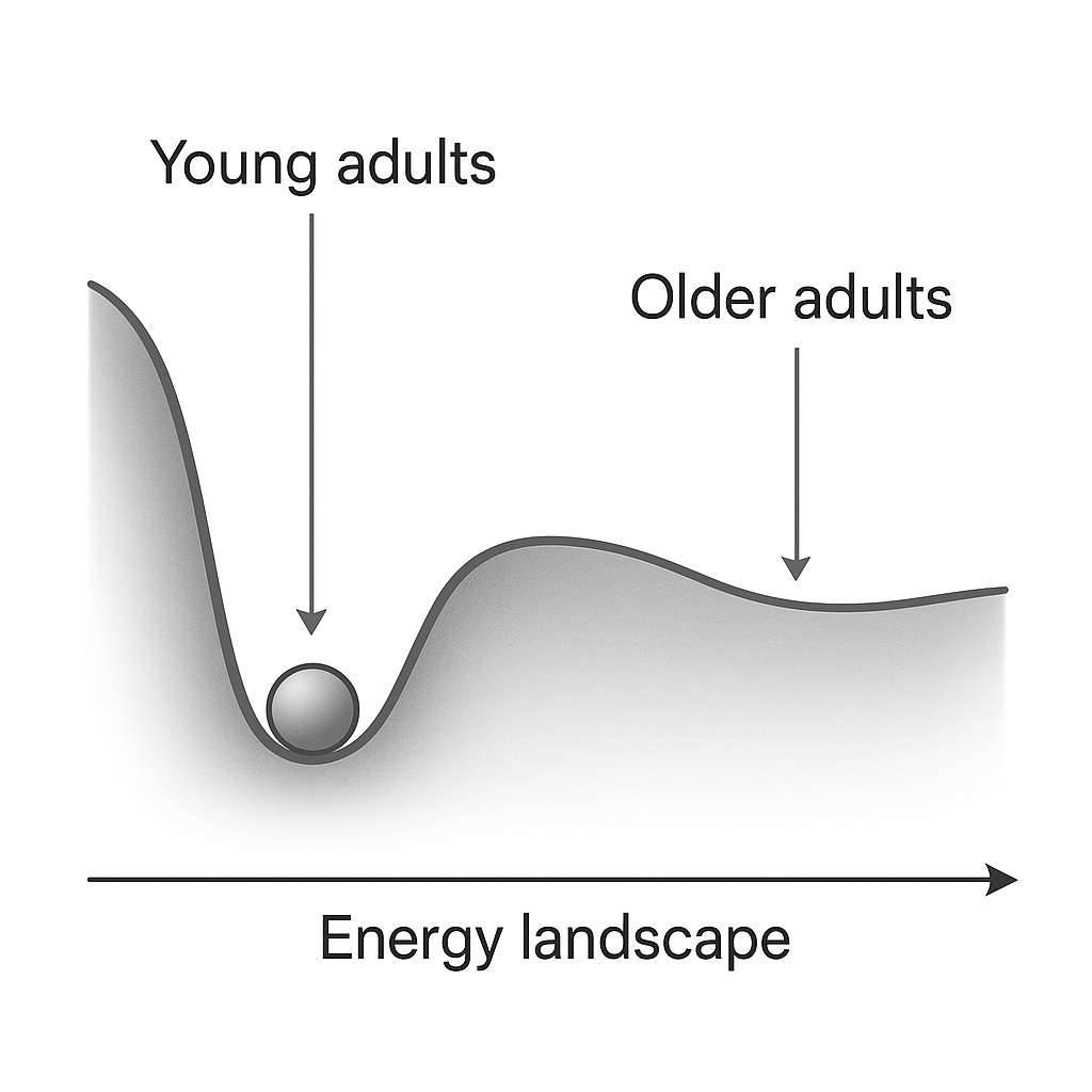
Figure 1: Simple visualization of energy landscape change with age. In young adults, perturbations (disease, DNA damage, etc...) roll back quickly towards the minimum, while in the older system the basin is shallower, making fluctuations persist and drift further from the minima. Generated with ChatGPT.
For instance, if we take a large population, young adults will cluster tightly around physiological norms such as 60-70 bpm, glucose near ~85 mg/dL, and low inflammatory markers. Older individuals will not only have a shifted baseline (higher glucose for instance), but a much broader spread across these dimensions with some drifting towards hypertension, others towards metabolic dysregulation, reflecting flatter and more weakly coordinated physiological basin.
Several quantitative questions follow naturally:
1. How steep is the basin?
2. Can we measure curvature and entropy from the data?
3. What happens to the youthful attractor with age?
4. Is aging drift directional or random?
5. Does curvature decrease with age?
6. Does the organism maintain memory of its initial configuration?
7. Does the system’s effective dimensionality change with age?
My goal is to build a coherent framework of tools that is able to answer these questions and allow to systematically interrogate and engineer living systems.
A key requirement for such framework is that it should reliably model how different levels of biological organization behave with age. In principle, it should be able to apply whether you are looking at epigenetic drift, heart rate variability, or any other micro/macro biomarkers. The key assumption is that different biomarker types give us different projections of the same underlying dynamical system.
In this blog I will practically apply my framework to the following human datasets:
1. Physiological data (NHANES) - 4k+ variables such as blood pressure, heart-rate variability, liver enzymes, blood glucose, and other clinical biomarkers that capture high level state of the organism.
2. Methylation data (GSE55763, GSE87571) - genome wide CpG methylation of peripheral blood representing long-term regulatory state. Methylation is a chemical tag a cell adds to DNA to control how genes are expressed.
3. Transcriptomic data (CD4+ subset of syn51197006) - single cell RNA seq reflecting fast cell level fluctuations of gene activity.
These three layers give us a comprehensive view into several levels of biological scales, allowing for a comprehensive hypothesis evaluation.
I want to note that I am not trying to propose another theory of aging here. My interest lies in proposing new ways we can holistically evaluate aging without speculating of its origins (for now). I believe aging needs more frameworks independent of molecular specifics. Whether data comes from transcriptomes, methylomes, or clinical patients — same geometric quantities should apply.
A physics based framework for aging
Based on the discussion above, the first step is obvious: let’s measure the shape of that landscape directly from data.
We can not observe the energy function itself, but we can estimate it indirectly from the population statistics. Probability distributions give us an ability to measure geometry thanks to their log-density properties that encode the landscape’s shape.
If youth corresponds to a well shaped Gaussian valley, then changes in the mean and covariance of those clouds tell us how the basin shifts, stretches, and flattens with age.
So instead of asking “Which genes go up or down?” we ask a more geometric question:
How does the probability distribution of system states deform as we move away from youth?
Here, we follow one of the fundamental insights from physics which states that systems tend to spend time in low-energy states (stable). Think of a marble in a bowl. As you put a ball at the rim, it will roll down to the bottom. Formally:
where the E(z) is the energy of a state z. We can further rewrite this as E(z)=-log p(z), where energy is simply negative log probability. From this, high probability states are low energy (stable), and rare states are high energy (unstable).
When we perturb a system (move it away from energy minimum), the system pulls with a restoring force which is the negative gradient of the energy.
Next, if we Taylor expand the energy near its minimum, the distribution becomes locally Gaussian
H is a Hessian matrix, which can be practically approximated by the inverse covariance of the system.
1. Eigenvectors of H are principal directions of curvature.
2. Eigenvalues of H are stiffnesses along those directions (small eigenvalues correspond to soft modes where its easy for the system to deform). Think of a stiff spring which barely stretches vs a soft spring that easily stretches.
3. Variance is reciprocal of the stiffness.

Figure 2: Imaginary energy landscape for a ball in a basin. Steep slopes (large curvature) correspond to small variance and flat regions correspond to large variance. Intuitively, a system will prefer to drift along the flatter regions since it requires little energy change, leading to fluctuations being naturally larger in those dimensions. Vector points along the soft mode of the landscape.
Having this framework, we then build a coordinate system where youth becomes the origin and unit of scale.
If we take youthful adults (for the sake of my experiments age <30) and compute their μ_Y and covariance ΣY. Then transform every sample z into whitened coordinates:
The operation does two beautiful things
1. Youthful state becomes centered and isotropic - N(0,I)
2. Every other donor is expressed in youth units and deviation from youth mean measured in standard youth variability.
So to summarize, whitening by the youthful state defines a coordinate system where every deviation of older adults is measured in youth units.
Note that each data point z does not represent an individual cell, but a donor level aggregate, which is a statistical summary of that donor’s molecular or physiological state. Practically, we group donors into age bins and treat each bin as one point. This avoids ill-conditioned matrices since the number of features per donor exceeds the number of observations. In addition, we work with principal components rather than raw features to make the computation tractable.
In this youth space, we can now talk about drift, dispersion, and curvature in comparable terms across data.
Quantifying drift and Dispersion
Once we are in the whitened space, we can express each donor by a Gaussian N(μ_d, Σ_d) Next, we introduce squared 2-Wasserstein distance W_2^2 between that donor and youth which breaks neatly into two interpretable parts:
1. Translation measures how far donor’s mean shifted from youthful center
2. Shape measures how covariance has deformed relative to identity
W₂ is naturally used here as distance between Gaussians because it combines mean displacement and covariance deformation (the two variables that define basin geometry). In a nutshell, it describes how far and how broadly each donor’s state has moved in the energy landscape.
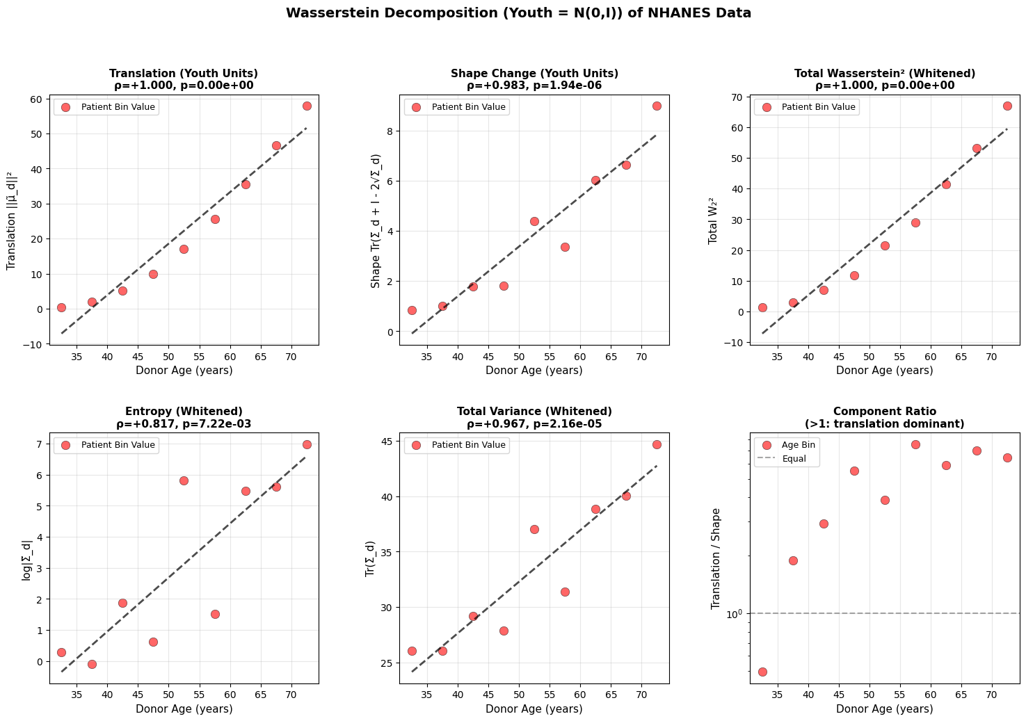
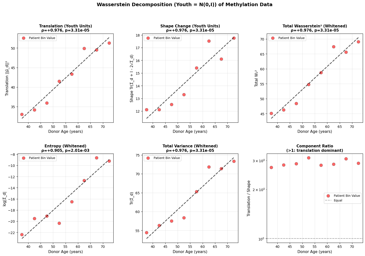
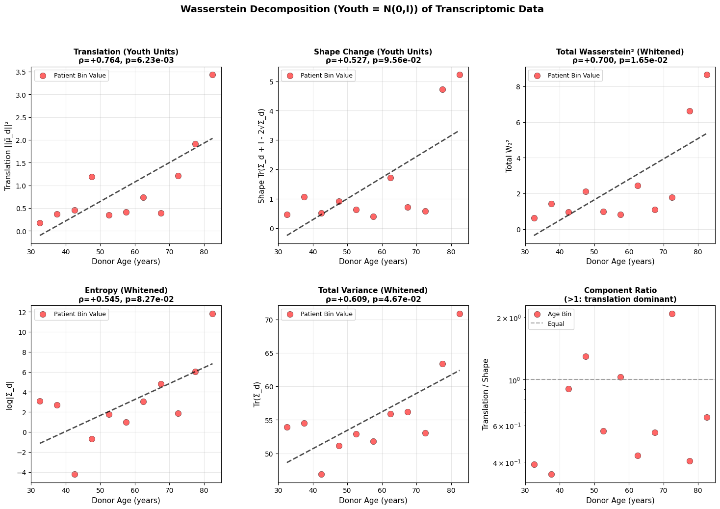
Figure 3: Wasserstein distance applied to aging dynamics across biological scales. Age-related changes in (a-c) translation, shape, and total Wasserstein distance in youth-whitened space for physiological (top block), epigenetic (middle block), and transcriptomic (bottom block) data. Translation captures directional drift from the youthful mean, while shape measures covariance deformation. (d-f) Entropy and variance evolution showing progressive state space expansion with age. All measurements in youth-standardized units where young donors are centered at N(0,I).
Both translation and shape increase with age. Entropy and total variance rise monotonically, showing that older organisms occupy a broader region of state space. Based on the epigenetic and physiology data, aging does not resemble purely random diffusion where variance increases equally in all directions, but rather a deformation that is dominant along a preferred trajectory. This is what we will explore in the next section.
A roughly linear increase in variance is a hallmark of stochastic (random–walk or diffusion–like) processes, which was also reported by Pyrkov et al. (2021). One implication is that the organism undergoes stochastic fluctuations around a drifting baseline, which is compatible with damage-based aging theories (Gladyshev, 2016).
There is also an interesting dynamic between translation and shape change in the methylation and physiology data. For example, heart rate variability decreases predictably with age in virtually everyone (deterministic trajectory), even as the variance around this trend increases (shape change). We all go down the same slope, but at slightly different angles and speeds. However, this clean interpretation breaks down at the transcriptomic level, where technical noise makes it unclear whether the underlying biology is truly more stochastic or if we’re simply hitting the resolution limits of current sequencing technologies.
Is Aging Directional or Random?
If every donor’s drift vector points in the same direction, aging is coherent: we all slide down the same slope of the landscape. If the directions scatter, it’s diffusive with noise dominating, and the system meandering rather than flowing.
To test this, we collect each donor’s whitened mean and compute
1. Consensus direction:
2. Each donor’s projections:
3. Off axis residual
Intuitively, we identify the dominant direction of change across all donors (u*), then compute if each donor moving along this shared path (captured by projection s_d), or are they scattering in random directions (measured by residual r_d)
Afterwards, we ask
1. Does s_d correlate with age?
2. Does r_d stay flat?
3. How concentrated are the direction vectors?
4. How straight is the path through age ordered means?
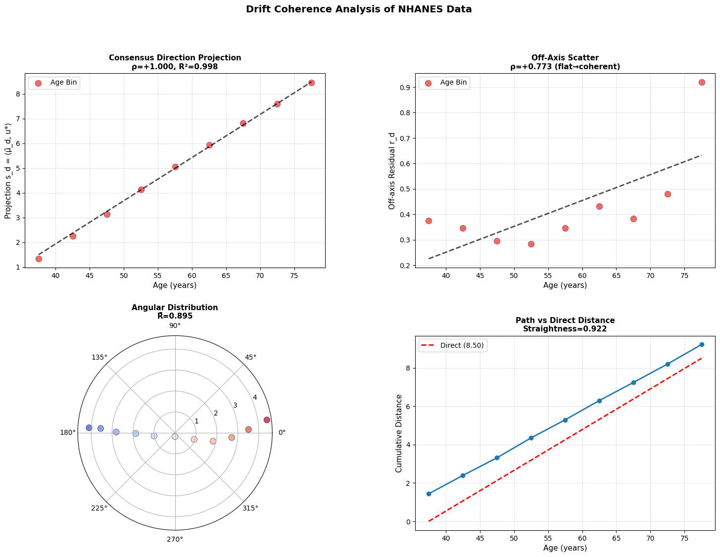

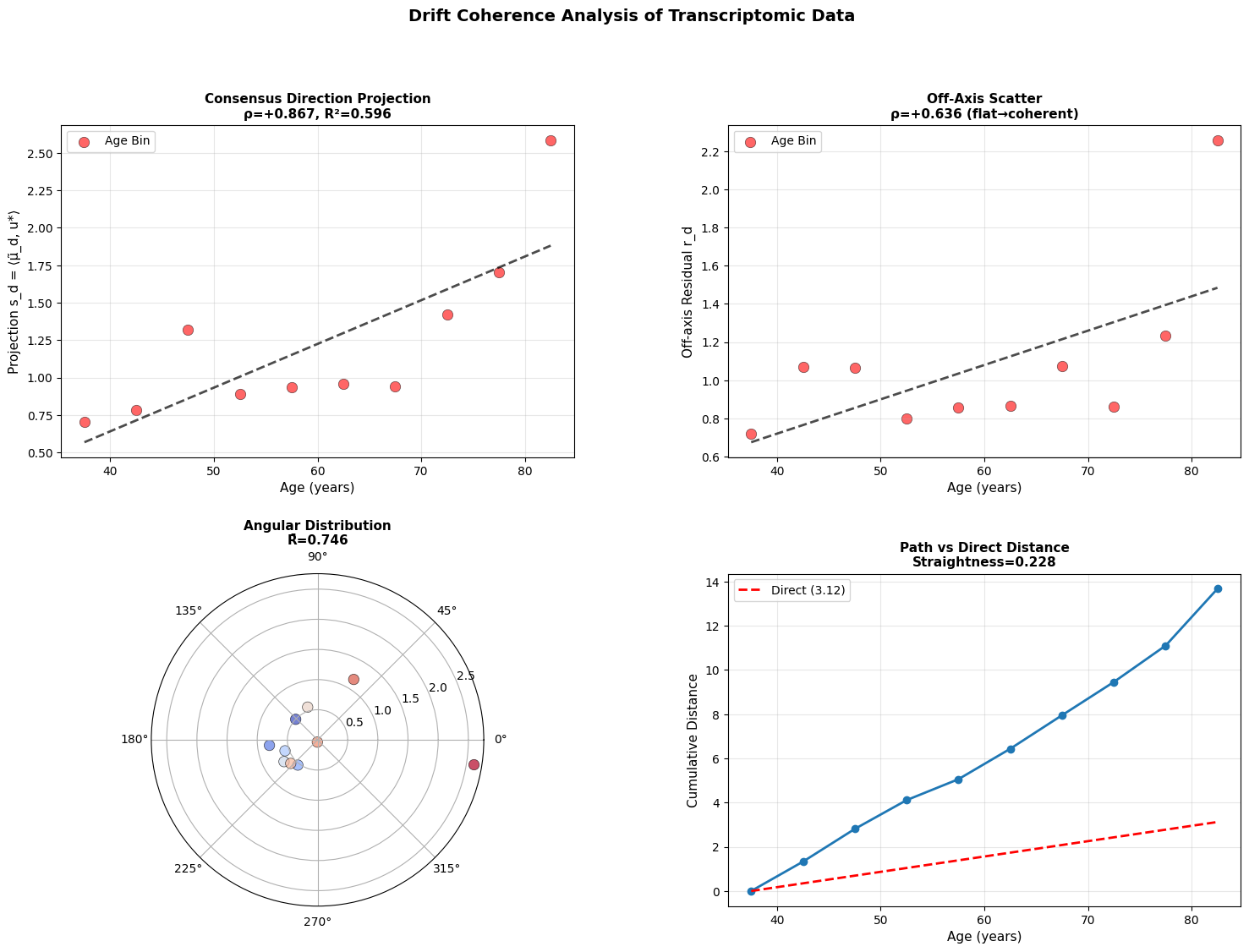
Figure 4: Aging follows a coherent trajectory. (a) Projection of donor states onto consensus aging direction shows strong correlation with age across modalities. (b) Off-axis residuals remain relatively flat, showing coherent rather than diffusive drift. (c) Angular distribution in polar projection reveals concentration around consensus direction. (d) Cumulative path distance versus direct distance demonstrates trajectory straightness.
While there is work showing that epigenetic clocks may be reproduced by accumulating stochastic variation (Meyer, 2024), the data above does not support purely stochastic aging. Instead, we see that methylome changes along a coherent low-dimensional trajectory, aligning strongly with consensus direction. This is consistent with manifold like aging dynamics reported in other models (Horvath, 2013; Snir et al., 2016; Farrell et al., 2020; Lapborisuth et al., 2022; Lu et al., 2023).
Across modalities, aging appears directional but progressively less coordinated at smaller biological scales. Macroscopic physiology drifts coherently, epigenetic states mostly follow, and cellular transcriptomes are less stable suggesting that aging begins as an organized global relaxation that fragments into local, noise-driven drift.
But in the section above we have just concluded that aging might be a stochastic drift due to the linear variance increase? Thermodynamics tells us that both observations could be true at the same time.
Adiabatic drift in thermodynamics states that fast stochastic variances equilibrate quickly, while slow variables evolve deterministically along a slow manifold. This results random fluctuations averaging out, and a coherent large-scale drift remaining. Analogously, we could consider a noisy cellular transcriptional state to average into a slow and deterministic trajectory of organismal level change that happens along a repeatable manifold.
Critical Slowing and Stability
So far we have looked at how systems drift from the youthful attractor and how its overall variance expands. The next question is to check how the underlying stability of that attractor changes with age. To do that, we will look at the flattest direction with the highest variance, where the curvature is the smallest, thus easier for the organism to deform along.
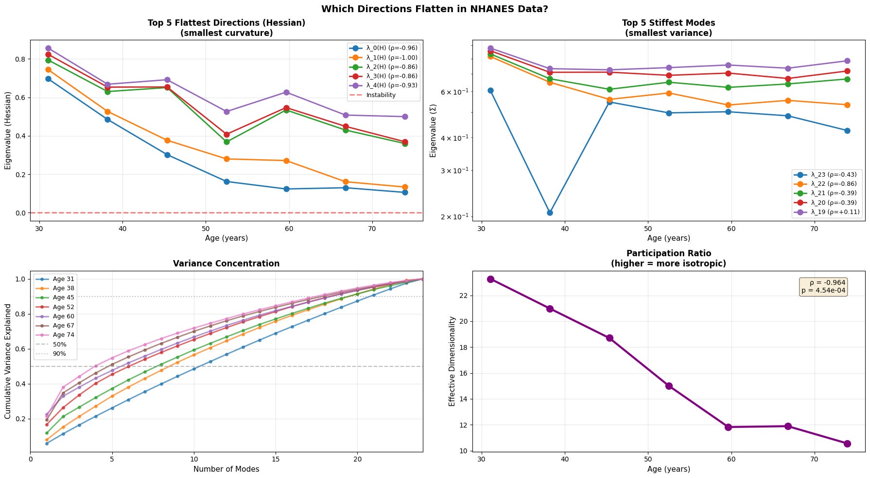
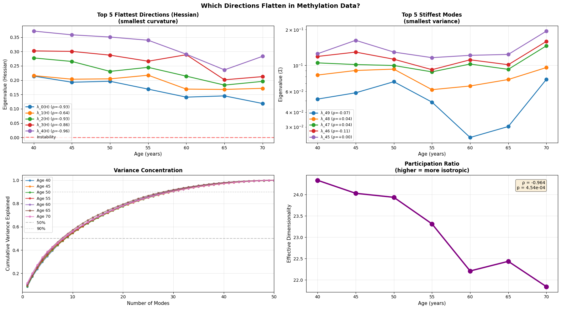
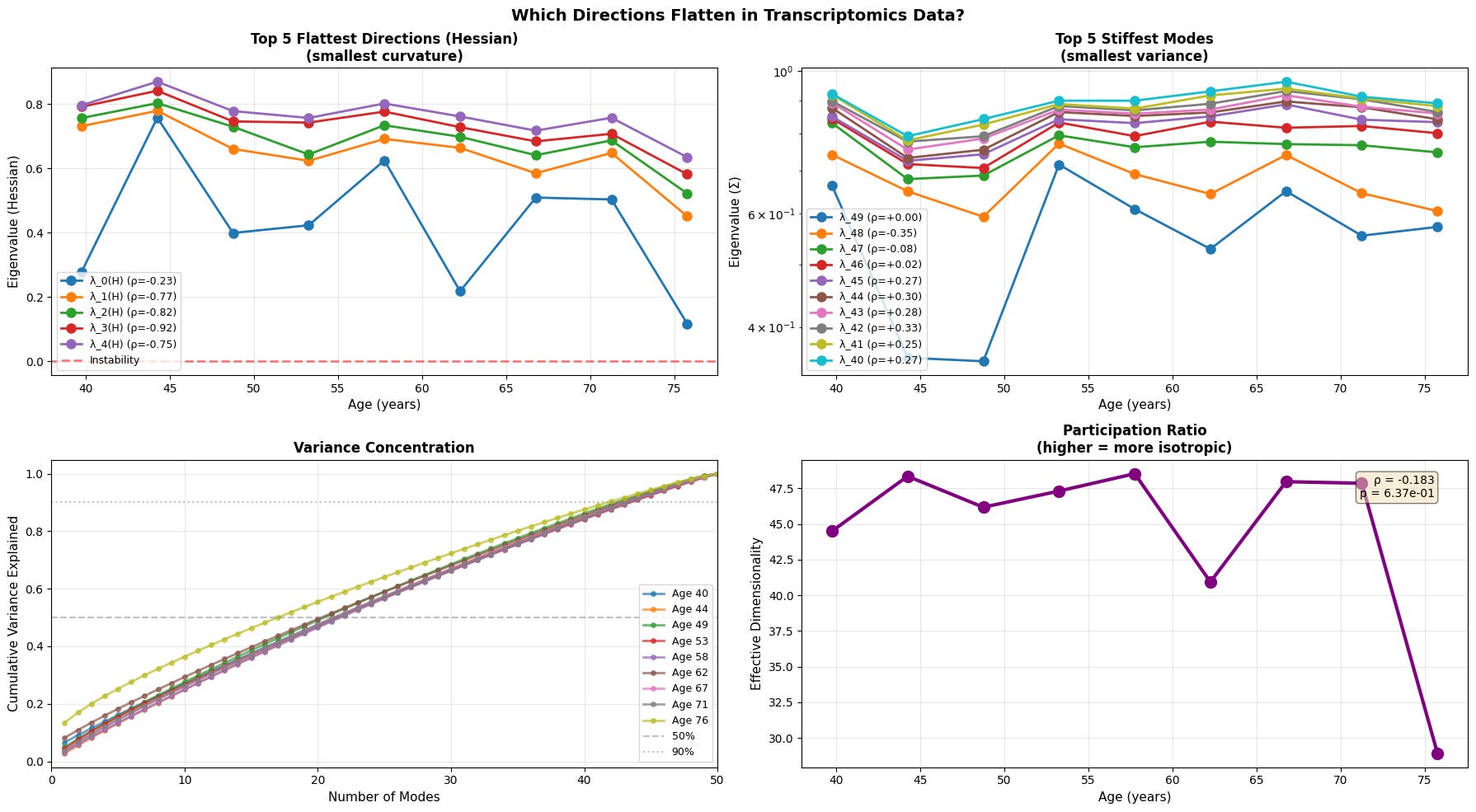
Figure 5: Anisotropic landscape flattening reveals selective loss of stability along soft modes. (a) Evolution of the five flattest directions (smallest Hessian eigenvalues) demonstrates progressive loss of curvature, with physiological data showing the clearest trend toward instability (red dashed line at λ=0). (b) The five stiffest modes (smallest variance) remain relatively stable or show inconsistent patterns (c) Variance concentration curves reveal that older individuals require fewer modes to explain the same proportion of total variance (d) Participation ratio (effective dimensionality) decreases with age.
With age, the softest directions of the energy landscape grow even softer, while the system gradually loses its participation ratio (a measure of effective dimensionality/isotropy). This means that the motion becomes intensified in certain directions and less evenly distributed. Notably, we see that the transcriptomic data is once again noisy with an abrupt fall in effective dimensionality at older age.
This is a textbook example of a system approaching a separatrix. Near a separatrix softest eigenvalues approach zero, and the valley slowly becomes a ridge, where even small fluctuations that once were easy to restore persist and push system into adjacent basin. In short, this phenomenon is a characteristic of resilience loss.
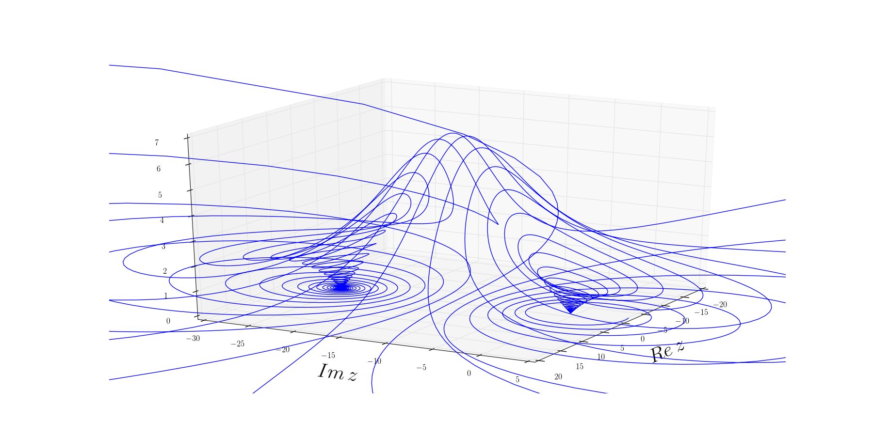
Figure 6: Visualization of a generic separatrix. As curvature along the saddle flattens (eigenvalue approaches 0), even small fluctuations can push the system from its original basin into the adjacent one, showing a loss of resilience with age. Source.
Kogan et al. (2015) proposed that long-lived species such as the naked mole rat remain youthful because their gene-regulatory networks lie on the stable side of a separatrix, maintained by high repair efficiency and low gene network connectivity. The flattening of soft modes we observe here could be an empirical example of humans crossing into the unstable region of stability. This perspective is also consistent with Promislow et al. (2022) who argues that that aging across biological, ecological, and psychological systems is fundamentally characterized by a decline in resilience (the ability to resist or recover from perturbations).
Predicting Future State
Do the softest directions (highest variance/lowest curvature) at age n-1 predict where the system will actually move by age n? Does the system mostly just move along the directions that are most favorable to it (a.k.a directions of least resistance)?
This is important since soft modes could simply be a data artifacts without having any causal power for aging.
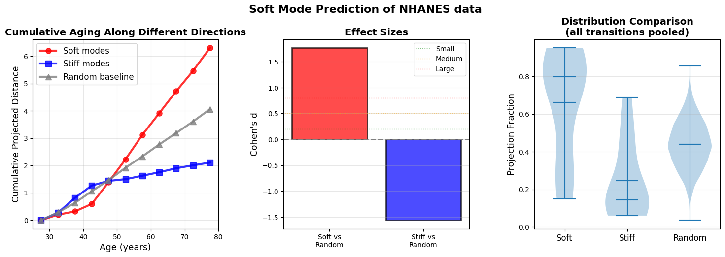
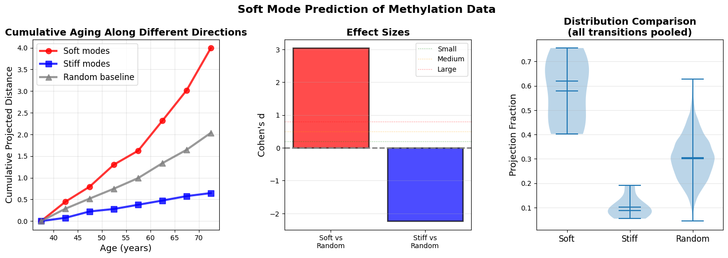
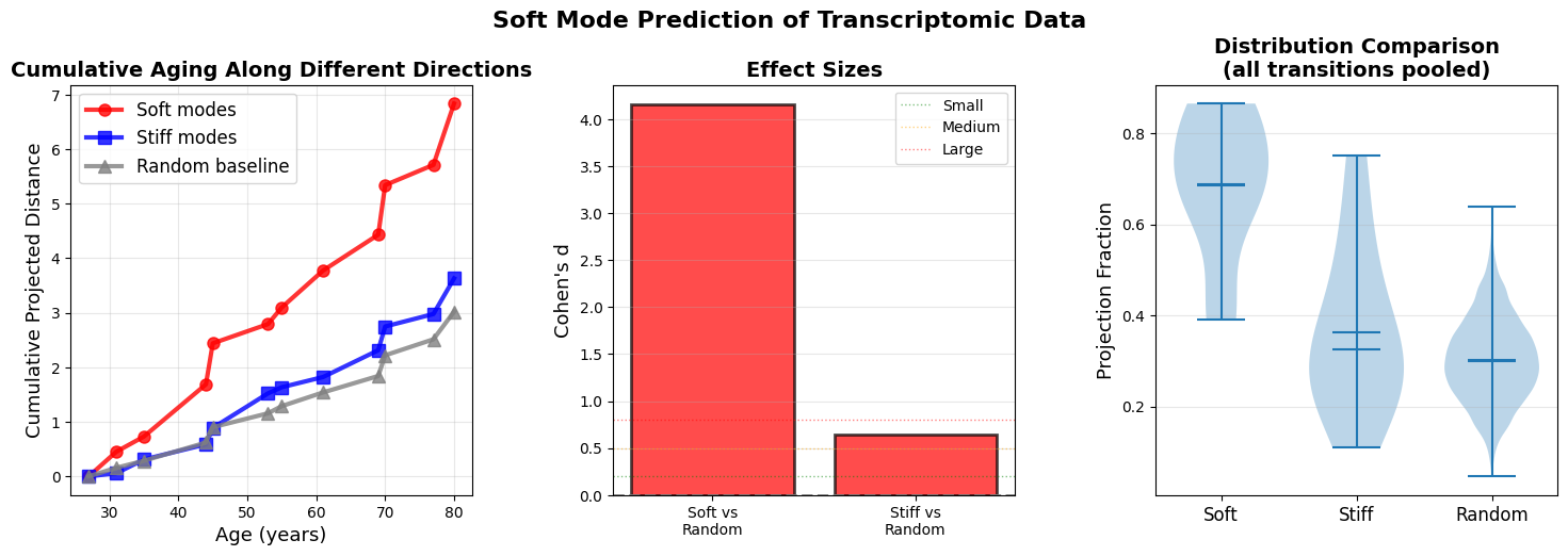
Figure 7: Soft modes at age n-1 predict aging trajectory to age n (a) Cumulative projected distance reveals that aging predominantly accumulates along soft mode directions (red). (b) Effect sizes (Cohen’s d) quantify the predictive power of soft modes over random directions. (c) Distribution of projection fractions for all ages across all n-1 to n transition.
Cumulative projected distance shows that aging predominantly accumulates along soft mode directions (top 10% highest-variance principal components, red), with stiff modes (bottom 10% lowest-variance PCs, blue) and random directions (gray) capturing even less displacement. The divergence strengthens at older ages when landscape anisotropy increases. The results support a gradient-flow interpretation where organisms ages along paths of least resistance defined by the local covariance structure.
Discussion
I have presented an outline of a simple framework how an engineer may think about aging. This framework is based on approximating the energy landscape of a living system and analyzing how it moves along the soft and stiff modes. The core findings are that:
There is a gradual flattening of the organism’s attractor basin with age.
Flattening is anisotropic and is occurring along soft modes.
These soft modes predict future aging trajectories, validating the mechanistic interpretation.
Indeed soft modes have been greatly explored in complex systems. Soft modes have been shown before to unify concepts from biophysics to microbial ecology. Russo et al. (2024) recently showed that soft modes unify concepts from protein allostery to microbial ecology. In gene regulatory networks, Furusawa et al. (2018) demonstrated that systems naturally evolve to channel perturbations along soft modes, regardless of whether the organism has previously encountered that specific perturbation. Kaneko (2024) has unified the concepts of variability, adaptability, and evolution ocuring along the soft modes of the system. Specifically, noise among genetically identical individuals shows where the system can flex (variability), that same direction is used for plastic adaptation within lifetime in response to environmental change, and evolution later fixes those changes genetically through evolvability. I believe soft modes are not a mathematical trick, but an evolutionary feature!
Why would evolution produce systems that age along predictable soft modes?
Russo et al. (2024) theorized that organisms perform unsupervised learning on their environment through selection. Over generations organisms distill the highly dimensional space of possible perturbations into a few important dimensions that matter for fitness while stiffening the ones that do not matter. There are two evolutionary reasons. First, organism must be stable. Mathematically, this corresoponds to stiffening most degrees of freedom and leaving only few soft modes. At the same time evolution selects for plasticity, which means that the organism should be able to adapt to new changes in its environment. This tradeoff realistically gives a low dimensional surface for all regulatory changes. Just 50 principal components capture ~25% of transcriptomic variance despite thousands of genes, 24 components explain ~ 90% of variance of 4k+ physiological features, and 50 principal components explain ~40% of methylome which contains hundreds of thousand sites. There is a small range of body temperatures or gene expression states that do not lead to a catastrophic organismal failure. The success of epigenetic clocks using just a few hundreds of CpG sites has also proved this low dimensionality.
Through this lense, we can look at aging as organism “forgetting” the adaptation of their environment as it drifts in the state space. Aging is the system sliding and diffusing along the very channels it was designed to be flexible in.
What about practical interventions?
This framework suggests two distinct targets for intervention: translation (drift from youth) and dispersion (loss of homeostatic precision). While related, these may require different intervention approaches. Speculatively, epigenetic reprogramming might reverse translation by resetting the system’s position in state space, while fixing genomic instability might prevent dispersion by maintaining landscape curvature. The observation that soft modes predict future movement suggests that we need to make sure that interventions that we design specifically address these directions.
Weaknesses of the framework
The framework heavily relies on modeling donor-level states as multivariate Gaussians which assumes local quadratic structure of the energy landscape, unimodal distributions, and linear covariance structures. I used traditionally interpretable tools like Wasserstein distance, but we can also use deep learning to model non-linear dynamics. For example, due to the noisy nature of transcriptomic data, I have been developing energy based deep learning models for transcriptomic trajectories, which show consistent results with the framework above. Here are a few early sneak peaks:
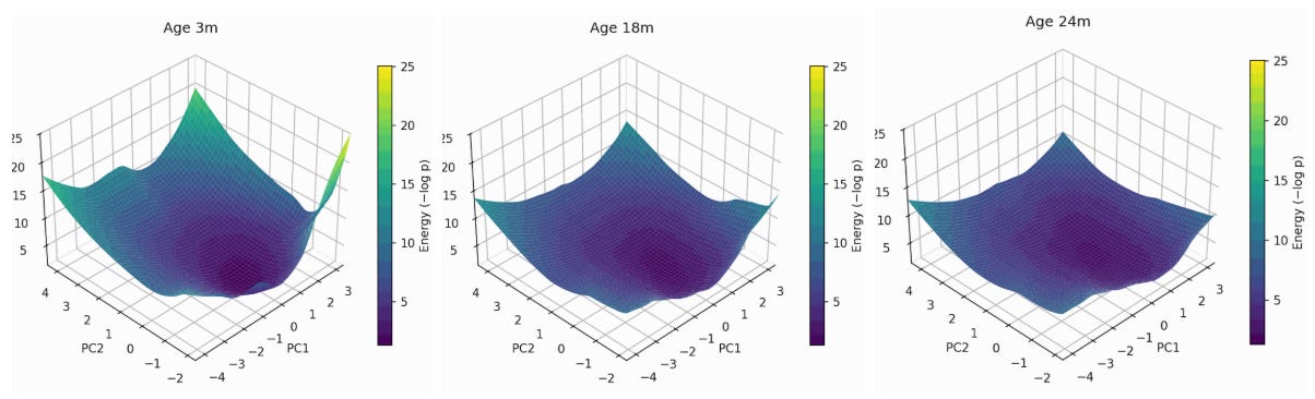
Figure 8: Energy landscape flattening of mouse Myeloid cells transcriptome. Shown at 3->18->24 months of mouse age, projected onto the first two principal components of gene expression, with the z-axis representing the energy of each state (higher energy less likely the state is). You can see expansion along a soft mode which is in the positive direction of PC2 and the middle of PC1
Figure 9: Human CD4+ cell aging landscape remodelling projected onto the first two principal components of gene expression, with the z-axis representing the energy of each state (higher energy less likely the state is).
I will revisit these modelling approaches in future posts.
Another weakness of the framework that I have presented is that covariance estimation is notoriously unstable in high dimensions. I tried to mitigate this with Ledoit–Wolf shrinkage, but relatively small donor counts in the datasets make the results susceptible to noise.
There is a lot of noise in the transcriptomic data which could be due to insufficient samples or CD4+ cell composition shift with age (though I measured the effect to be insignificant and tried to regress it out)
Future Directions
Can we apply this framework to measure someones landscape flatness as a biomarker more reliable compared to methylation clocks? Could we use to predict who will respond to rejuvenation therapies?
Do rejuvenation interventions like rapamycin, partial reprogramming, and plasma exchange actually re-steepen the energy landscape? Do they translate it?
How do we further quantify the important of the soft vs stiff modes in aging? How do we choose interventions that act along specific modes?
I think of biomedicine as an act of landscape engineering. Through both a quantitative framework for tracking aging and specific predictions for designing interventions I hope we can tackle aging more effectively.
Aged epigenomes are directly downstream of DNA breaks. Is there a similar link between translation and dispersion
Love this!